Parametric Tutorial

NOTE This notebook is not meant to teach statistics, but only demo how to run the py50 functions. There are plenty of resources available online. I particularly found introductory tutorials by DATAtab helpful.

The following page will show examples of parametric tests using the Stats() and Plots() modules of py50. There are many plot features available for py50, but they will not all be demoed here. Instead, to see all the plots available, take a look at the 006_statistics_quickstart. As py50 is built on top of Pingouin, additional examples with ANOVA tests can be found here.

[1]:

from py50 import Stats, Plots
import pingouin as pg

[2]:

## List Datasets available from Pingouin
# pg.list_dataset()

# Read Dataset
df = pg.read_dataset('penguins')

# Initialize Stats and Plots
stats = Stats(df)
plot = Plots(df)

print('List of Group names in Dataset:', df['species'].unique())
stats.show()

List of Group names in Dataset: ['Adelie' 'Chinstrap' 'Gentoo']

[2]:

	species	island	bill_length_mm	bill_depth_mm	flipper_length_mm	body_mass_g	sex
0	Adelie	Biscoe	37.8	18.3	174.0	3400.0	female
1	Adelie	Biscoe	37.7	18.7	180.0	3600.0	male
2	Adelie	Biscoe	35.9	19.2	189.0	3800.0	female
3	Adelie	Biscoe	38.2	18.1	185.0	3950.0	male
4	Adelie	Biscoe	38.8	17.2	180.0	3800.0	male

Data Distribution

The data distribution is important to determine patterns that may show up in the dataset. For example, it can also tell you how often a value may occur, the shape of the data, variability of a value, etc.

py50 includes two tests that can help analyze the dataset.

Normality. This will test if the dataset follows normal distribution - i.e. a bell-shape curve.
Homoscedasticity. This will test for the “spread” or consistency of the dataset along a regression model.

[3]:

# Test for normality
stats.get_normality(value_col='body_mass_g', group_col='species').round(3)

[3]:

	W	pval	normal
species
Adelie	0.981	0.032	False
Chinstrap	0.984	0.561	True
Gentoo	0.986	0.234	True

[4]:

stats.get_homoscedasticity(value_col='body_mass_g', group_col='species').round(3)

[4]:

	W	pval	equal_var
levene	NaN	NaN	False

ANOVA

Several tests, parametric and non-parametric, are available in py50. The functions use the “get_x” format, where x is the name of said test. Here, the One-Way ANOVA script will be demoed. The final table will be a Pandas.DataFrame object.

[5]:

anova = stats.get_anova(value_col='body_mass_g', group_col='species')
anova

[5]:

	Source	ddof1	ddof2	F	p_unc	np2	significance
0	species	2	339	343.626275	2.892368e-82	0.669672	****

Tukey

py50 comes with several post-hoc tests. Again, this can be called using the same ‘get_x’ phrase. As the above ANOVA test show significance between the Hair color group, a Tukey test will be performed.

[6]:

tukey = stats.get_tukey(value_col='body_mass_g', group_col='species').round(4)
tukey

[6]:

	A	B	mean_A	mean_B	diff	se	T	p_tukey	hedges	significance
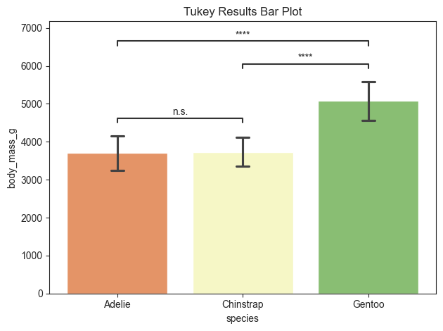
0	Adelie	Chinstrap	3700.6623	3733.0882	-32.426	67.5117	-0.4803	0.8807	-0.0739	n.s.
1	Adelie	Gentoo	3700.6623	5076.0163	-1375.354	56.1480	-24.4952	0.0000	-2.8602	****
2	Chinstrap	Gentoo	3733.0882	5076.0163	-1342.928	69.8569	-19.2240	0.0000	-2.8753	****

The tukey results can be plotted as follows:

The parameters for all plots in py50 are created to be as similar as possible. For each plot, there is also an option to “return_df”. This parameter will output the calculated dataframe that was used to create the plot. Users can use this to compare to the plot generated using the Stats() module to check for any inconsistencies.

[7]:

title = 'Tukey Results Bar Plot'

plot.barplot(test='tukey', value_col='body_mass_g', group_col='species', palette='RdYlGn', title=title, fontsize=30,
             return_df=True)

[7]:

(           A          B       mean_A       mean_B         diff         se  \
 0     Adelie  Chinstrap  3700.662252  3733.088235   -32.425984  67.511684
 1     Adelie     Gentoo  3700.662252  5076.016260 -1375.354009  56.147971
 2  Chinstrap     Gentoo  3733.088235  5076.016260 -1342.928025  69.856928

            T       p_tukey    hedges significance
 0  -0.480302  8.806666e-01 -0.073946         n.s.
 1 -24.495169  1.443290e-14 -2.860201         ****
 2 -19.223978  1.443290e-14 -2.875327         ****  ,
 <statannotations.Annotator.Annotator at 0x119fe7a60>)

../_images/tutorials_007_parametric_example_11_1.png

Welch ANOVA

Welch ANOVA is used for when the Homoscedasticity is false. In other words, if the datasets does not look consistent. The get_welch_anova() function can be tested usign the same Penguin dataset used above.

[8]:

# welch = stats.get_welch_anova(data, value_col='body_mass_g', group_col='species').round(4)
welch = stats.get_welch_anova(value_col='body_mass_g', group_col='species')
welch

[8]:

	Source	ddof1	ddof2	F	p_unc	np2	significance
0	species	2	189.478413	317.572267	3.093701e-61	0.669672	****

Games-Howell Post-Hoc Test

Again, after the ANOVA test, a post-hoc test should be used to tell significance between groups. Games-Howell can be used to handle situations with inconsistent datasets - i.e. Homoscedasticity is false.

[9]:

gameshowell = stats.get_gameshowell(value_col='body_mass_g', group_col='species')
gameshowell

[9]:

	A	B	mean_A	mean_B	diff	se	T	df	pval	hedges	significance
0	Adelie	Chinstrap	3700.662252	3733.088235	-32.425984	59.706437	-0.543090	152.454796	0.850154	-0.073946	n.s.
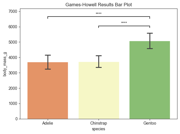
1	Adelie	Gentoo	3700.662252	5076.016260	-1375.354009	58.810929	-23.386028	249.642554	0.000000	-2.860201	****
2	Chinstrap	Gentoo	3733.088235	5076.016260	-1342.928025	65.102843	-20.627794	170.404362	0.000000	-2.875327	****

The post-hoc results can be plotted using py50. Her there are specific pairs denoted for plotting. This would remove the pairs that have no significance (n.s.). If the return_df=True, then the returned table will only contain the pairs annotated on the plot.

[10]:

title = 'Games-Howell Results Bar Plot'
pairs = [('Gentoo', 'Chinstrap'), ('Adelie', 'Gentoo')]

plot.barplot(test='gameshowell', value_col='body_mass_g', group_col='species', palette='RdYlGn', title=title,
             fontsize=30, return_df=True, pairs=pairs)

[10]:

(           A       B       mean_A      mean_B         diff         se  \
 1  Chinstrap  Gentoo  3733.088235  5076.01626 -1342.928025  65.102843
 0     Adelie  Gentoo  3700.662252  5076.01626 -1375.354009  58.810929

            T          df  pval    hedges significance
 1 -20.627794  170.404362   0.0 -2.875327         ****
 0 -23.386028  249.642554   0.0 -2.860201         ****  ,
 <statannotations.Annotator.Annotator at 0x11a29c5b0>)

../_images/tutorials_007_parametric_example_17_1.png

Repeated Measures

Repeated measures is used to analyze within-subjects or within-groups factors. Can be used when the subjects are measured under different conditions or time points. Examples for the get_rm_anova() function uses the ‘rm_anova’ dataset from pingouin as follows:

[11]:

repeated_m = pg.read_dataset('rm_anova')
repeated_m.dropna(subset=['Gender'], inplace=True)

rm_stats = Stats(repeated_m)
rm_plots = Plots(repeated_m)
rm_stats.show()

[11]:

	Subject	Gender	Region	Education	DesireToKill	Disgustingness	Frighteningness
0	1	Female	North	some	10.0	High	High
1	1	Female	North	some	9.0	High	Low
2	1	Female	North	some	6.0	Low	High
3	1	Female	North	some	6.0	Low	Low
4	2	Female	North	advance	10.0	High	High

[12]:

repeated_measures = rm_stats.get_rm_anova(value_col='DesireToKill', within_subject_col='Disgustingness',
                                          subject_col='Subject')
repeated_measures

[12]:

	Source	ddof1	ddof2	F	p_unc	ng2	eps	significance
0	Disgustingness	1	91	11.876684	0.000862	0.025827	1.0	***

Pairwise tests for repeated measures

The guidelines found on Pingouin suggest pairwise_tests(). py50 warps this function in the get_pairwise_rm() function. The results can also be used to plot hte results.

NOTE: Depending on the data, it may also be feasible to use the Tukey test.

[13]:

pairwise_test = rm_stats.get_pairwise_rm(value_col='DesireToKill', within_subject_col='Disgustingness',
                                         subject_col='Subject')
pairwise_test

[13]:

	Contrast	A	B	Paired	Parametric	T	dof	alternative	p_unc	BF10	hedges	significance
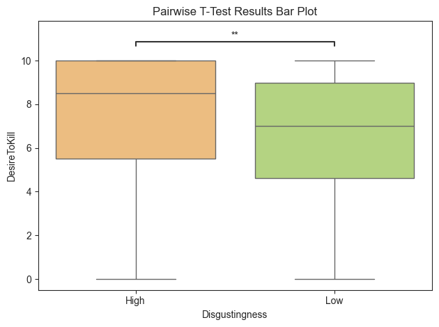
0	Disgustingness	High	Low	True	True	3.446257	91.0	two-sided	0.000862	26.262	0.322536	***

[14]:

title = 'Pairwise T-Test Results Bar Plot'

rm_plots.boxplot(test='pairwise-rm', value_col='DesireToKill', group_col='Disgustingness', subject_col='Subject',
                 palette='RdYlGn', title=title, fontsize=30, return_df=True)

[14]:

(         Contrast     A    B  Paired  Parametric         T        dof  \
 0  Disgustingness  High  Low   False        True  2.595165  360.18469

   alternative     p_unc   BF10    hedges significance
 0   two-sided  0.009841  2.899  0.271888           **  ,
 <statannotations.Annotator.Annotator at 0x119ce0c10>)

../_images/tutorials_007_parametric_example_23_1.png

Mixed ANOVA

Mixed ANOVA can be used to analyze data with mixed design - both within and between group factors. The function uses the py50 standard as seen in the above examples. The example here will use the ‘mixed_anova’ dataset from Pingouin.

[15]:

data = pg.read_dataset('mixed_anova')
mixed_stats = Stats(data)
mixed_plot = Plots(data)

mixed_stats.show()

[15]:

	Scores	Time	Group	Subject
0	5.971435	August	Control	0
1	4.309024	August	Control	1
2	6.932707	August	Control	2
3	5.187348	August	Control	3
4	4.779411	August	Control	4

[16]:

mixed = mixed_stats.get_mixed_anova(value_col='Scores', group_col='Group', within_subject_col='Time',
                                    subject_col='Subject')
mixed

[16]:

	Source	SS	DF1	DF2	MS	F	p_unc	np2	eps	significance
0	Group	5.459963	1	58	5.459963	5.051709	0.028420	0.080120	NaN	*
1	Time	7.628428	2	116	3.814214	4.027394	0.020369	0.064929	0.998751	*
2	Interaction	5.167192	2	116	2.583596	2.727996	0.069545	0.044922	NaN	n.s.

The guidelines found on Pingouin suggest pairwise_tests(). That can also be used. But depending on the dataset, it may be more prudent to use the tukey test. That is easy to use, as we have seen above. The Tukey test will be performed and the corresponding barplot() will be generated.

[17]:

pairwise_test = mixed_stats.get_tukey(value_col='Scores', group_col='Group')
pairwise_test

[17]:

	A	B	mean_A	mean_B	diff	se	T	p_tukey	hedges	significance
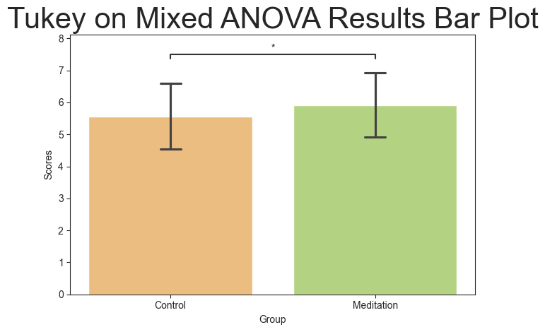
0	Control	Meditation	5.567851	5.91618	-0.348328	0.152115	-2.289903	0.0232	-0.339918	*

[18]:

title = 'Tukey on Mixed ANOVA Results Bar Plot'

mixed_plot.barplot(test='tukey', value_col='Scores', group_col='Group', palette='RdYlGn', title=title, titlesize=30,
                   return_df=True)

[18]:

(         A           B    mean_A   mean_B      diff        se         T  \
 0  Control  Meditation  5.567851  5.91618 -0.348328  0.152115 -2.289903

    p_tukey    hedges significance
 0   0.0232 -0.339918            *  ,
 <statannotations.Annotator.Annotator at 0x11a5aa020>)

../_images/tutorials_007_parametric_example_29_1.png