py50 Quickstart

The following details how to get up and running using py50. These funcitons take in simple parameters to plot the dose-response curves. There are three plotting options - Single Curve, Multi Curve, and Grid Plot.

[1]:

import pandas as pd
from py50 import Calculator, PlotCurve

Calculate Relative and Absolute IC50

[2]:

# Read in dataset
example = pd.read_csv('../dataset/single_example.csv')

calc_data = Calculator(example)  # Instantiate dataframe into the Calculator class
calc_data.show()

[2]:

	Compound Name	Compound Conc	% Inhibition 1	% Inhibition 2	% Inhibition Avg
0	Drug 1	100000.0	90	94	92
1	Drug 1	33300.0	97	89	93
2	Drug 1	11100.0	86	89	88
3	Drug 1	3700.0	81	88	84
4	Drug 1	1240.0	63	70	67

[3]:

# Perform calculation
# If only relative IC50 needed, can use the calc_data.calculate_ic50() function instead.
calc_data = Calculator(example)
calculation = calc_data.calculate_ic50(name_col='Compound Name', concentration_col='Compound Conc', response_col=['% Inhibition 1', '% Inhibition 2'])
                                                # response_col='% Inhibition Avg')
calculation

[3]:

	compound_name	maximum	minimum	ic50 (nM)	hill_slope
0	Drug 1	92.865625	-8.210081	429.962039	1.024522

Scale results to pIC50

If IC50 is not your cup of tea, you can quickly scale the values into pIC50 values. This is done using the calculate_pic50() function. It will calculate absolute IC50, but will append two additional columns for hte relative pIC50 and absolute pIC50.

[4]:

calculation = calc_data.calculate_pic50(name_col='Compound Name', concentration_col='Compound Conc',
                                        response_col='% Inhibition Avg')
calculation

[4]:

	compound_name	maximum	minimum	relative ic50 (nM)	absolute ic50 (nM)	hill_slope	relative pIC50	absolute pIC50
0	Drug 1	92.854405	-7.640226	439.824243	584.73401	1.040878	6.356721	6.233042

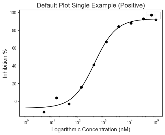
Single Curve

[5]:

single = pd.read_csv('../dataset/single_example.csv')
plot_data = PlotCurve(single)

figure1 = plot_data.curve_plot(concentration_col='Compound Conc',
                               response_col='% Inhibition Avg',
                               title='Default Plot Single Example (Positive)',
                               name_col='Drug 1',
                               xlabel='Logarithmic Concentration (nM)',
                               ylabel='Inhibition %',
                               legend=True)

../_images/tutorials_001_quickstart_8_0.png

[6]:

plot_data.show()

[6]:

	Compound Name	Compound Conc	% Inhibition 1	% Inhibition 2	% Inhibition Avg
0	Drug 1	100000.0	90	94	92
1	Drug 1	33300.0	97	89	93
2	Drug 1	11100.0	86	89	88
3	Drug 1	3700.0	81	88	84
4	Drug 1	1240.0	63	70	67

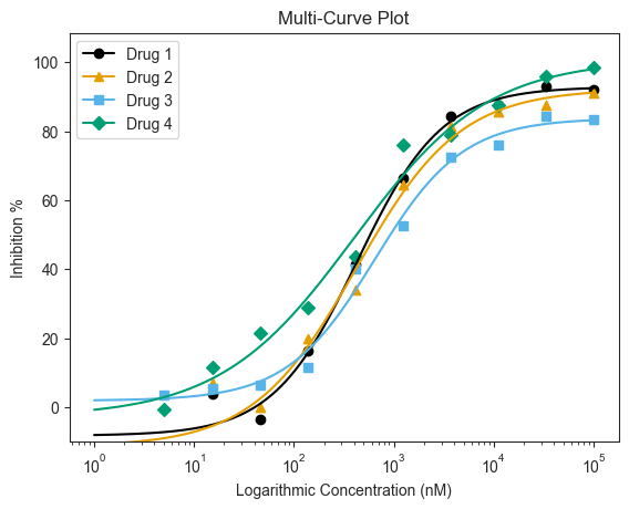
Multi-Curve

[7]:

# Read in Dataset
multi = pd.read_csv('../dataset/multiple_example.csv')

# Instantiate dataframe into the PlotCurve class
plot_data = PlotCurve(multi)

# Optional to inspect table
# plot_data.show()

[8]:

figure3 = plot_data.multi_curve_plot(name_col='Compound Name',
                                     concentration_col='Compound Conc',
                                     response_col='% Inhibition Avg',
                                     title='Multi-Curve Plot',
                                     xlabel='Logarithmic Concentration (nM)',
                                     ylabel='Inhibition %',
                                     legend=True,
                                     ymin=-10,
                                     markersize=10)

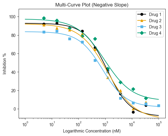
../_images/tutorials_001_quickstart_12_0.png

[9]:

# For negative slope
# Read in Dataset
multi = pd.read_csv('../dataset/multiple_example_negative.csv')

# Instantiate dataframe into the PlotCurve class
plot_data = PlotCurve(multi)

figure4 = plot_data.multi_curve_plot(name_col='Compound Name',
                                     concentration_col='Compound Conc',
                                     response_col='% Inhibition Avg',
                                     title='Multi-Curve Plot (Negative Slope)',
                                     xlabel='Logarithmic Concentration (nM)',
                                     ylabel='Inhibition %',
                                     legend=True,
                                     ymin=-10)

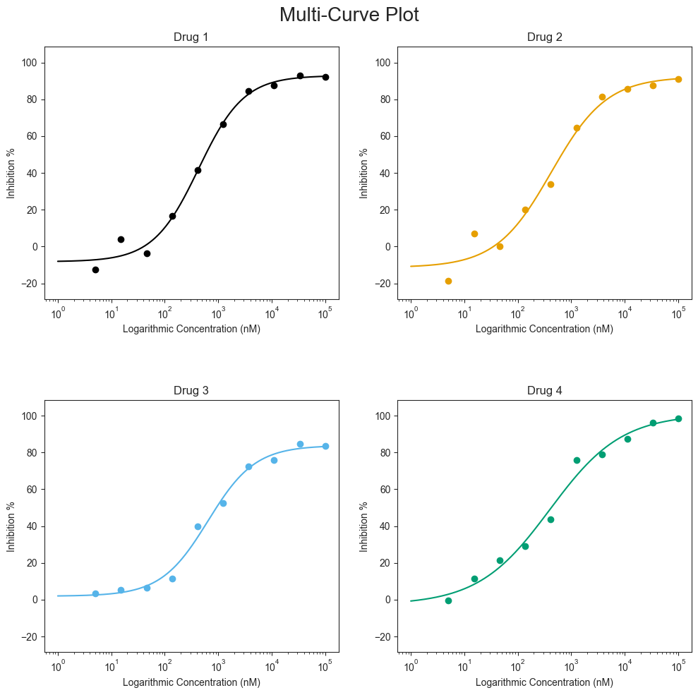
../_images/tutorials_001_quickstart_13_0.png

Grid Plot

[10]:

# Read in Dataset
grid = pd.read_csv('../dataset/multiple_example.csv')

# Instantiate dataframe into the PlotCurve class
grid_plot = PlotCurve(grid)

# Optional to inspect table
grid_plot.show()

[10]:

	Compound Name	Compound Conc	% Inhibition 1	% Inhibition 2	% Inhibition Avg
0	Drug 1	100000.0	90	94	92.0
1	Drug 1	33300.0	97	89	93.0
2	Drug 1	11100.0	86	89	87.5
3	Drug 1	3700.0	81	88	84.5
4	Drug 1	1240.0	63	70	66.5

[11]:

figure5 = grid_plot.grid_curve_plot(name_col='Compound Name',
                                    concentration_col='Compound Conc',
                                    response_col='% Inhibition Avg',
                                    title='Multi-Curve Plot',
                                    xlabel='Logarithmic Concentration (nM)',
                                    ylabel='Inhibition %',
                                    conc_unit='nM',
                                    figsize=(10, 10))

../_images/tutorials_001_quickstart_16_0.png